Big O notation
23 Nov 2020What is the Big O Notation?
The Big O notation is a way to measure the performance of an algorithm. The performance is measured in two ways, time and space. Time is how long the algorithm takes to run and space is how much memory the algorithm uses. The Big O notation is written like this O(n). Inside the parentheses is how the algorithm run time or space will grow as the input size grows. In this article I will cover some of the most common run times and more about the Big O notation.
Time Complexity
Time complexity describes the runtime of an algorithm. The runtime can be broken down into three different sections: best, worst and average case. Below I will cover each of these cases and the runtime of the example below:
def findIndex (arr, item):
    for i in range(len(arr)):
        if arr[i] == item:
            return i
- Best case- The best case runtime would be O(1). This would occur when the first element in the array is equal to the inputted item.
- Worst case- The worst case would be O(n). The worst possible case would be if the last item in the array was equal to the item inputted. This would mean the whole array would need to be iterated through.
- Average case- The average runtime would also be O(n). This is because in the average case part of the array is still going to need to be iterated over.
The best case scenario isn’t commonly used in the programming industry since it doesn’t provide much helpful information. The best case scenario may be O(1). But knowing this doesn’t help prepare for the average and worst case scenarios. Also it doesn’t help when trying to improve the algorithm’s efficiency because if the best case runtime is O(1) then this can’t be improved upon.
The average and worst case runtime are often the same. The average case runtime gives a better understanding on how efficient the algorithm is going to be. The worst case runtime will indicate if the current algorithm is efficient enough to handle any input given.
Space Complexity
Space complexity describes how much memory is taken by an algorithm. In the iterative function below the space complexity would be O(n). This is because the memory used grows proportionally with the input size. Space complexity also applies to the call stack on a recursive algorithm. If a recursive function is called n times then the space complexity would also be O(n). Examples:
# Iterative function O(n) space
def square (arr):
    squared = []
    for i in range(len(arr)):
        sum = arr[i] * arr[i]
        squared.append(sum)

    return squared
# Recursive function O(n) space
def sum (num):
    if num <= 0:
        return num

    return num + sum(num-1)
Drop Constants and Non Dominant Terms
When describing a runtime of an algorithm constants and non dominant terms are dropped. This is because they do not affect how a runtime scales. An example of where a constant would be dropped is a double-looped algorithm. Although the algorithm has two separate loops the runtime would still be considered O(n) instead of O(2n) since the runtime of the algorithm is still going to grow linearly.
An example of where a non dominant term would be dropped is an algorithm with a nested loop as well as a singular loop. This algorithm’s runtime would be O(n²) instead of O(n² + n). As mentioned above this will be dropped since the extra loop does not affect how the runtime scales. Note this only applies to subtraction and addition of non dominant terms, multiplication and division of non dominant terms is still valid e.g O(n*log(n)).
Runtime Comparisons
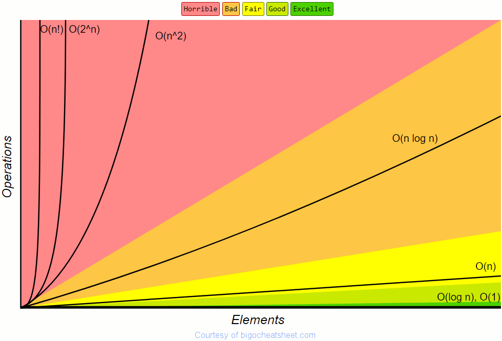
The chart below displays the rate of growth for common runtimes as their input size increases. This chart should make it easier to visualize the growth rate of each runtime.

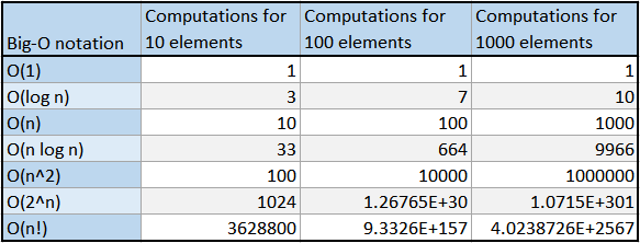
The table below shows how many computations occur for each runtime with input sizes of: 10, 100, and 1000. This table should help demonstrate the computational growth of each runtime.

Different Runtimes
This section will cover the 7 different runtimes in the chart above in order from quickest to slowest. In each example I will give a brief description of the runtime and a code example to help visualize what x runtime may look like.
The first runtime is O(1) complexity and can also be referred to as a constant runtime. If an algorithm has a constant runtime the maximum amount of operations won’t change even if the input size changes. An example of a O(1) runtime would be a Stack Insertion:
def push (self, data):
    node = StackNode(data)
    node.next = self.top
    self.top = node
    self.size += 1

# Time O(1)
# Space O(n)
The next runtime is O(log(n)). This is also known as a logarithmic runtime. This means on each loop the input size will roughly half. An example of this would be Binary Search:
def targetIndex (arr, target):
    left = 0
    right = len(arr)
    index = int(right / 2)

    while left <= right:
        if arr[index] == target:
            return index

        if arr[index] < target:
            left = index + 1
        else:
            right = index - 1

        index = (right - left) // 2 + left

    return -1

# Time O(log(n))
# Space O(1)
The third runtime is O(n) and this is also called a linear runtime. This means the amount of iterations / calls will grow with the input size. An example of this would be searching for an element in a Linked List:
def find (self, item):
    node = self.root

    while node:
        if node.data == item:
            break

    node = node.next

    return node

# Time O(n)
# Space O(1)
The next runtime is O(n*log(n)) which is also referred to as a quasilinear runtime. An example of this Merge Sort:
def mergeSort (arr, startIndex, endIndex):
    if startIndex != endIndex:
        middle = int((startIndex + endIndex) / 2)
        mergeSort(arr, startIndex, middle)
        mergeSort(arr, middle+1, endIndex)
        return merge(arr, startIndex, arr[startIndex:middle+1], arr[middle+1:endIndex+1])

def merge (arr, index, left, right):
    leftStart = 0
    leftEnd = len(left) - 1
    rightStart = 0
    rightEnd = len(right) - 1

    while leftStart <= leftEnd and rightStart <= rightEnd:
        if left[leftStart] < right[rightStart]:
            arr[index] = left[leftStart]
            leftStart += 1
        else:
            arr[index] = right[rightStart]
            rightStart += 1

        index += 1

    while leftStart <= leftEnd:
        arr[index] = left[leftStart]
        leftStart += 1
        index += 1

    while rightStart <= rightEnd:
        arr[index] = right[rightStart]
        rightStart += 1
        index += 1

    return arr

# Time O(n*log(n))
# Space O(n)
The fifth runtime is O(n²) and can also be called a quadratic runtime. This means the input squared is roughly the estimated amount of iterations / calls which will be made for this algorithm. An example of this is Bubble Sort:
def bubbleSort(arr):
    count = 1

    while count < len(arr):
        for i in range(len(arr) - count):
            c = arr[i]
            n = arr[i + 1]

        if c > n:
            temp = c
            arr[i] = n
            arr[i + 1] = temp

        count += 1

    return arr

# Time O(n²)
# Space O(1)
The penultimate runtime is O(2ⁿ) and is also known as an exponential runtime. This runtime is fairly slow and won’t be able to handle big inputs. An example of this would be the Fibonacci Sequence:
def fib(n: int) -> int:
    if n <= 1:
        return n

    return fib(n - 1) + fib(n - 2)

# Time O(2ⁿ)
# Space O(n)
The final runtime is O(n!) and this can also be referred to as a factorial runtime. This is an extremely slow runtime but sometimes may be the only option depending on the problem. An example of this would be a function which generates all permutations of a string:
def permutations(head, tail=''):
    if len(head) == 0:
        print(tail)
    else:
        for i in range(len(head)):
            permutations(head[:i] + head[i+1:], tail + head[i])

# Time O(n!)
# Space O(n! * n)
Summary
Having a good understanding of the Big O notation is essential when looking to improve your understanding of data structures and algorithms. This knowledge helps us make better decisions when writing algorithms and selecting the best data structure for that algorithm. If you want to look through the code example click here. If you are looking for extra resources on the Big O notation check the sections below.
Resources
Cracking the Coding Interview 6th Edition (Pages 38 - 60)